The post Lamar Jackson: Looking ahead by looking back first appeared on 'CATS STATS.
]]>Jackson’s season was extremely impressive statistically. While he was about average in passing yards during the regular season (22nd in the league with 3,127), he led the NFL in passing touchdowns with 36 and had the ninth best completion percentage. It is also worth mentioning that Jackson put up these numbers on only 265 passing attempts, placing him just 27th in the league. Where Jackson really shone, however, was his rushing: he rushed for an NFL QB record 1,206 yards and 7 touchdowns, while also breaking his own record in rush attempts from last season. Jackson’s 1,206 yards were more than twice as many as second place Kyler Murray, who finished the season with 544 rushing yards. One can gain a better sense of just how special Jackson’s season has been by comparing his numbers to the historical rushing record. The former record for rushing yards by a quarterback was 1,039—set by Michael Vick in 2006. The gap between Jackson’s record-setting season and Vick’s former record is larger than the gap between the second and fifth place (902) spots on the same list. In addition, the new record marks a 16% increase over Vick’s original record.
Jackson is only in his second year in the NFL and is very likely headed for a bright future. As a young dual-threat quarterback, what might that future look like? Given that Jackson has such a unique profile and has already broken the single season rushing yards record, attempting to use past statistics to project his growth seems unlikely to be effective. What can work however is to look at the longevity of other dual-threat quarterbacks. Most dual-threat quarterbacks seem to have a peak performance window of 4-5 years, after which their rushing ability declines, and they need to rely more on their passing game. However, the sample size for these is minuscule in comparison to traditional pocket quarterbacks.
Often, rushing is considered to be the most punishing part of a dual-threat quarterback’s career. This article on Yahoo! Sports, however, found that a quarterback is hurt while scrambling approximately once every 91.7 plays. By comparison, a quarterback being sacked was hurt once every 92.5 plays, and a quarterback struck while releasing a pass was hurt once in every 67.1 plays. These numbers demonstrate that rushing may not be nearly as dangerous for quarterbacks as has been conventionally thought. This means that Jackson’s record-setting number of rushing attempts could actually serve to prolong his career and rushing ability. In addition, Jackson’s passing numbers for this season were incredible, both on their own and compared to his first season. Jackson is still young, so it is not unreasonable to think that his passing game will continue to improve with time. Even if Jackson’s legs start to decline sooner than hoped, he still clearly has the potential to be one of the most impressive and exciting players in the league. It is important to remember that, in spite of being an MVP frontrunner and NFL touchdown leader, this was Jackson’s first full season as a starter. With the level of ability that he has demonstrated both in his passing and rushing game, it is safe to say that Jackson’s future is looking bright.
The post Lamar Jackson: Looking ahead by looking back first appeared on 'CATS STATS.
]]>The post Parity in the NBA first appeared on 'CATS STATS.
]]>Traditional metrics are more indicative of style of play than of competitive balance. A team with a high pace of play could appear better than they actually are in many areas such as rebounds, steals, points, and assists, all of which would be inflated by the team’s high pace. At the same time, a team that is smaller and more focused on shooting will likely generate fewer rebounds, even if they are one of the best teams in the league.
Advanced statistics, like player efficiency rating or box plus minus (a per 100 possessions metric that uses box scores and team overall performance to estimate a player’s level of impact), allow us to see a more complete picture. In particular, these statistics are less influenced by the individual style of the team.
There is one additional problem in setting up this data: rookies. Rookies are one of the most unpredictable factors in the NBA. There is no prior relevant data that can be easily transferred to the NBA to make predictions about their performance, since many players’ college stats and first-year stats look wildly different in regards to both traditional and advanced metrics. Considering that, I have made the decision to exclude rookies and their potential numbers from the team averages. This will have an impact on teams such as New Orleans, who are planning to feature Zion Williamson as their star player from the beginning, but most teams will not be significantly impacted by this exclusion. This is even more true in the case of high-level playoff teams, where rookies rarely see meaningful minutes.
To find statistical evidence of an increase in parity, I decided to use last year’s data organized into two data sets.
The first set was the final rosters at the end of last season. The second set was last year’s data, reorganized using this season’s rosters. Then, I took the standard deviations for the advanced stats for each roster. In order to try and account for differences in playing time, I took one standard deviation using all players and a second using only players that played over 400 minutes played last season. In theory, the year that has more parity will, in general, have lower standard deviations when comparing the group of all teams in the NBA, demonstrating a possible way to demonstrate whether or not there actually is more parity in the league this year.
The advanced statistics I will be focusing on are VORP (value above replacement player), PER (player efficiency rating), offensive, defensive, and overall BPM (box plus minus), offensive, defensive, and total WS (win shares, a box score based calculation that estimates how many wins that player was responsible for over the course of the season), as well as WS/48 (win
shares per 48 minutes). As a note, offensive win shares are also sometimes referred to as GA-SW.
When comparing the statistics using all players on the 2018 and 2019 rosters, there is variation, but a general trend indicates that there is in fact more parity this year compared to last.
In the “All players” category, standard deviation was lower in 2019 than in 2018 in PER, DWS, WS/48, OBPM, DBPM, and BPM. Standard deviation was lower in 2018 in OWS, WS, and VORP. In the “400+ minutes played” category, standard deviation was lower in 2019 in OWS, DWS, WS, WS/48, OBPM, DBPM, BPM, and VORP. Only PER had a lower standard deviation in 2018 than in 2019.
Overall, and especially in the “400+ MP” group, there seems to be more parity this year than last. There are exceptions, most notably PER as the single outlier in the 400+ group, but not enough to reverse the trend. While it is essentially impossible to measure the comparative power of each advanced statistic, the overall strength of the trend suggests an increase in parity.
That being said, an increase in parity does not mean that every team is now competing on the same level. For example, although the standard deviation for VORP is lower in comparison to last year, when comparing the average team VORP’s from 2018 and 2019, Cleveland remains significantly behind the majority of teams. In all four data groups, Cleveland has a negative VORP, and is the only team in this situation in either of the 2019 groups. While the top of the graph, included below, has balanced out considerably, Cleveland remains in the same negative position as last year.


Cleveland’s case is also indicative of one of the potential flaws in this analysis, borne from using last year’s advanced statistics with this year’s rosters. As a team in the lottery, Cleveland’s goal is likely not to compete for an NBA championship, but to develop the players on their roster and the team as a whole. This means current statistics used as projections may be completely different from the numbers they actually put up. The roster may not even look like it currently does come the end of the season. This same issue is also true for teams with playoff aspirations, but it is less salient as development is less of a focus for them.
Additionally, many of the teams with a similar emphasis on development, such as the Knicks or the Grizzlies, have high-level rookie players. The impact of players like RJ Barrett and Ja Morant cannot be predicted with any accuracy and have therefore not been included in the calculations. This factor makes these rebuilding teams less likely to perform in accordance with their statistics. That being said, while the amount of variance may be greater for these teams, it should not be so much that the numbers used are irrelevant. Many players have semi-consistent levels of production across their careers, especially developing players who hit their ceiling. As such, the overall variance should not be so overwhelming that the overall accuracy is undercut.
Overall, several statistical indicators show more parity in the NBA than last season. 2019 has more statistics with lower standard deviation than 2018, and 2019 almost completely sweeps the “400+ MP” group, which is meant to show heavier weighting to players who will be more involved in the season. Parity is not perfect—there is still a large difference in many categories between playoff contenders and teams in the middle of a rebuild, but by the metrics used these distances are smaller than they were last year. So how will this look to fans?
Hopefully, fans see closer games, higher intensity, and more underdog wins. The Phoenix Suns so far have been outperforming expectations, and the Warriors will probably not find themselves winning by 20 points going into the fourth quarter nearly as often as they did last year. Only time will tell, but it looks like this season will be more intriguing than last season.
The post Parity in the NBA first appeared on 'CATS STATS.
]]>The post Usage Rates first appeared on 'CATS STATS.
]]>We examined the relationships among our variables by running a bivariate regression using usage rating and games played, and a multivariate regression that added minutes per game. The data supported our hypothesis, though not at a confidence interval of 90% or above. The underlying assumption is that a high level of involvement within a game as well as throughout the season for an individual player will likely be reflected in that player’s usage rating. More specifically, a high usage rating will likely be accompanied by above average playing time.
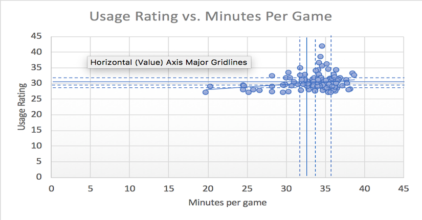
The independent variable, usage rating, identifies the most important players for each team. The dependent variables, minutes played per game and games played per season, measure a player’s involvement on the court. These measurements attempt to capture how a team tries to maximize the value of their key players through the time they spend on and off the court.
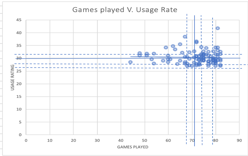
As expected, Figure 1 has a positively sloped trendline. Unexpectedly, Figure 2 has a slightly negative slope. We believe that this is indicative of the effect of usage rating on games played, because we focused on a sample of players whose teams attempt to maximize their utility in as many games as possible. We believe that if we expanded our sample size to all players in the league, the coefficient in Figure 2 would become positive (see Table 2).
The regression model can be expressed as follows:
Bivariate: Y = α0 + α1X1 + ε (1)
Multivariate: Y = α0 + α1X1 + α2X2 + ε (2)
where Y = usage rating, X1 = games played per season, and X2 = minute played per game.
| Y | X1 | X2 | |
| Mean | 30.34 | 71.94 | 33.489 |
| Standard Deviation | 2.5499 | 8.6335 | 3.6379 |
| Skewness | 1.4543 | -1.2411 | -1.6175 |
| Minimum | 26.9 | 44 | 19.7 |
| 25th Percentile | 28.8 | 68 | 32.2 |
| Median | 29.8 | 74 | 34.4 |
| 75th Percentile | 31.535 | 79 | 35.9 |
| Maximum | 41.7 | 82 | 38.7 |
| Correlation with Y | -0.03610 | 0.23457 | |
| Correlation with X1 | 0.11720 |
Likewise, we observed a negative regression coefficient, indicating a negative relationship between usage rating and games played. Initially, we hypothesized that the correlation between these two variables would be positive, as NBA teams will have more of an incentive to utilize players with high usage ratings in as many games as possible. However, the bivariate regression reflects the contrary: higher usage rating leads to a slightly lower number of games played. While this may hold true in some cases due to the risk for injury associated with higher usage rating, we believe this value may be inaccurate due to the low number of variables captured by the regression. This could be explained by omitted variable bias. Once we accounted for the control variable, minutes played per game, the regression coefficient for games played switched to a positive value.
Although we were able to capture the impact of the omitted variable bias in relation to minutes played per game, there are also several other omitted variables that could have a significant effect on this regression, including players’ health, sleep, and nutrition, and the front office’s influence on morale.
| Bivariate | Multivariate | |
| X1 | -0.00813 (0.02677) | 0.00129 (0.02744) |
| Control | N/A | 0.0641 (0.0448) |
| R2 | -0.00813 | 0.00131 |
Another limitation can be found in Table 2,
which displays very low R² values, meaning that our data was not very closely
clustered around our linear regression equation. We believe that this is
another indication of the high number of influential but not measurable omitted
variables when calculating sports statistics.
For example, we would expect players with a high defensive
workload to play fewer games, following the logic that an increased level of
involvement (on either end of the court) will lead to an increased risk of
injury, causing players to miss a few games over the course of the season.
Therefore, we would assume a negative correlation between usage rating and
defensive contribution.
Likewise, another potential omitted variable is the average number
of a team’s possessions per game. This statistic would reflect the pace at which
the team plays during a game, with a higher number of possessions indicating a
faster pace. We believe that a lower number of average possessions will lead to
both higher usage rating and higher games played, because the player will need
to use fewer possessions, and therefore less energy, to achieve the same usage
rating. This would also lower the risk for missing games, as we hypothesize
that greater amounts of play will lead to a greater risk for injury. Overall,
we would assume a negative correlation between the two: fewer team possessions
per game would likely increase usage
rating.
The outliers in our current sample are neither unexpected nor harmful to our results, and are
explainable. For example, unpredictable injuries explain our two largest
outliers for low games played, Chris Bosh and Kristaps Porzingis, each of whom
suffered season-ending injuries in multiple seasons. Tony Wroten, an outlier
for low minutes, spent the first half of the season coming off the bench before
excelling as a starter, leading him to have an unusually low number of minutes.
Russell Westbrook and James Harden, our two biggest outliers for usage rating, were
each tasked with being the sole major offensive force for his team.
We conclude that our results support our initial hypothesis: NBA
players with high usage ratings play both a high number of minutes per game and
a high number of games per season, though not all. The multiple regression
analysis supports this by demonstrating a positive correlation between usage
rating and games played, as well as usage rating and minutes played per game,
implying that all three variables move in the same direction. However, the
bivariate regression analysis displayed a negative correlation between usage
rating and games played, introducing some inconsistency to our data analysis.
Our analysis implies that, on average, NBA teams will maximize the playing time of individual players who possess high usage ratings, while ensuring some rest within a game or season to prevent major injuries. Knowing this can help organizations, opponents, and even fans to predict the type of roles and habits certain players may develop. To obtain more comprehensive results, similar research would need to be done with a much larger and more diverse sample of the league to account for the omitted variables that we were unable to capture. The results from such research would help to increase general understanding of the usage rating statistic, and further expand the realm of sports statistics.
This was written by Sam Lucas and Mary Ture.
The post Usage Rates first appeared on 'CATS STATS.
]]>